Kitabı oxu: «The Unlucky Investor's Guide to Options Trading»

The Unlucky Investor’s Guide to Options Trading

Julia Spina

Coauthored by Anton Kulikov

Foreword by Tom Sosnoff

Copyright © 2022 by tastytrade, Inc. All rights reserved.

Published by John Wiley & Sons, Inc., Hoboken, New Jersey.

Published simultaneously in Canada.

No part of this publication may be reproduced, stored in a retrieval system, or transmitted in any form or by any means, electronic, mechanical, photocopying, recording, scanning, or otherwise, except as permitted under Section 107 or 108 of the 1976 United States Copyright Act, without either the prior written permission of the Publisher, or authorization through payment of the appropriate per‐copy fee to the Copyright Clearance Center, Inc., 222 Rosewood Drive, Danvers, MA 01923, (978) 750‐8400, fax (978) 750‐4470, or on the web at www.copyright.com. Requests to the Publisher for permission should be addressed to the Permissions Department, John Wiley & Sons, Inc., 111 River Street, Hoboken, NJ 07030, (201) 748‐6011, fax (201) 748‐6008, or online at http://www.wiley.com/go/permission.

Limit of Liability/Disclaimer of Warranty: While the publisher and author have used their best efforts in preparing this book, they make no representations or warranties with respect to the accuracy or completeness of the contents of this book and specifically disclaim any implied warranties of merchantability or fitness for a particular purpose. No warranty may be created or extended by sales representatives or written sales materials. The advice and strategies contained herein may not be suitable for your situation. You should consult with a professional where appropriate. Further, readers should be aware that websites listed in this work may have changed or disappeared between when this work was written and when it is read. Neither the publisher nor authors shall be liable for any loss of profit or any other commercial damages, including but not limited to special, incidental, consequential, or other damages.

For general information on our other products and services or for technical support, please contact our Customer Care Department within the United States at (800) 762‐2974, outside the United States at (317) 572‐3993 or fax (317) 572‐4002.

Wiley also publishes its books in a variety of electronic formats. Some content that appears in print may not be available in electronic formats. For more information about Wiley products, visit our web site at www.wiley.com.

Library of Congress Cataloging‐in‐Publication Data is Available:

ISBN 9781119882657 (Hardcover)

ISBN 9781119882671 (ePDF)

ISBN 9781119882664 (ePub)

Cover Design and Image: © Cassie Scroggins

Author Photos: © Garrett Roodbergen

To Beth, Ken, and Joe Spina, as well as all the smaller, fuzzier Spinas that have joined us along the way

The ace‐ace‐nine is an inside joke at tastytrade and quite possibly the most annoying way to lose a hand of blackjack. Blackjack, for those unfamiliar with gambling, is a game between a dealer and player where the objective is to get closest to 21 without exceeding it. Face cards are worth 10 and aces are worth either 1 or 11. Imagine being at a blackjack table sitting pretty with 20, and the dealer is showing an ace. They confirm they don't have blackjack, turn over their second card and show another ace. The round is basically won and done because the dealer has a terrible hand, totaling 2 or 12, against your 20. The dealer draws their third card and reveals a nine, and by the time you've done the math, the house has already taken your chips.

Foreword

I've come a long way from my knuckle‐dragging pit trading days of the 1980s and 1990s. I take the wrapper off hot dogs when I eat them now, and I have also learned a few things about investing after 20 years of meeting people all over the country and teaching them how to trade. One crazy takeaway: Unlucky investors usually make the best traders. Why? Because anyone can get lucky and profit from a random investment, but in the small world of successful traders, the common denominator is quantitative skill. Another crazy takeaway: Anyone can learn these skills with access to the right information.

Way back when TD Ameritrade bought thinkorswim in 2009, I negotiated with every bit of leverage I had to personally keep the domain name, tastytrade.com. I had purchased the web address for $9.95 years earlier through GoDaddy, and I was convinced, just as I was with thinkorswim, that the name tastytrade would work. I have no idea why I loved tastytrade.com, but sometimes hunches just seem to work out. tastytrade's raison d'être was to fill the void in the financial media and offer up an untested, goodwill model built around raw, math‐based content. We've spent the last 10 years obsessively building client engagement by introducing complex financial strategies to retail investors. We still answer questions 24 hours a day and teach lessons from what we learned as market makers and software entrepreneurs: all for free. We truly are the guest who won't leave, but we believe that nonstop client engagement is core to motivating traders.

I have so many special memories from the last two decades, but one of my favorites was a strange trading story from an early 2001 trip to the desert. It was the first time we did a live trading show in Las Vegas, and a big trader at the event asked me how long it would take to get a fill on a large order using our platform. When I asked for his order, the client told me he wanted 10,000 spreads. This was before electronic spread executions existed, and I figured he was bullshitting me. But, as a show of good faith (and because I didn't want to back down), I told him we'd fill the order within one second. The client was convinced it wasn't going to happen, so I was pretty pleased when I told him, hand signal and all, that his order was filled in less than a second and the price improved by a nickel. We made asses of ourselves, but this is how it all began. Over the years, we continued to form unbreakable relationships with hundreds of thousands of amazing friends, traders, and investors. We gambled together, ate dinner together, had drinks at the bar, laughed when we made money, and cried when we lost money. We told jokes, embarrassed ourselves, humbled each other, and tortured our friends. We focused on building those relationships not only because it was a blast but because we also really saw how it motivated people to learn how to trade and participate in the market. It was key to the success of thinkorswim, and it inspired the founding of tastytrade.

When we started tastytrade, our proving ground was an old hip‐hop studio in downtown Chicago. It was a third‐floor walk‐up with a piano as the receptionist's desk and a drum set in the middle of the living room. Old album covers and broken musical instruments were everywhere, yet the energy was undeniable. Our research team consisted of a Guitar Hero champion in a hot dog suit, a few interns, and an ex‐market maker. Our mentor was a sports shock jock whose claim to fame was having sex on the 50‐yard line at Soldier Field, and to top it all off, we had hired a bunch of random comedians from Chicago's famed Second City. Thank God we knew how to trade because we had no clue how to do media. Even worse, I will never forget the day we decided to do HD quality video. I thought, “No way is that what I look like.” That's why tastytrade is so awesome because we figured out a totally new model of financial media when the odds were against us.

Lucky investors never figure things out because they never have to: They simply follow the herd and hope for the best. We refused to follow traditional financial media down the path of self‐promotion and financial irrelevance. We found smart people, fed them cheap lunches, made them work crazy hours, gave them free snacks, and mostly let them do their own thing. The result? We changed the world of strategic investing.

We knew early on that a book about options trading would add a new layer to our model of engagement and be a powerful tool for creating financial content. Eighteen years ago, I locked myself in our old conference room with one of our cofounders, and we tried to write a book. We hired a professional writer, cleared our schedules, and made the book a priority. Three days later and one and half pages in, we fired the writer and quit the book project to protect our friendship and the future of our firm. Fast forward to early 2021, and I was again bitten by the book bug, but this time, I knew I wasn't up to the task. I asked, as nicely as I am capable of, for two of our young, smart researchers to help. I said, “It's all yours.” Julia and Anton accepted the challenge, and they totally nailed it. I truly believe this is the most logical, informative, and comprehensive book on strategic options trading ever compiled. Unlucky investors can rejoice. No book will ever be a one‐size‐fits‐all holy grail for options trading, but The Unlucky Investor's Guide to Options Trading is the closest thing we have.

Tom Sosnoff

Preface

If the conditions are just right, extraordinary things happen when many individual pieces come together: Water molecules organize and form snowflakes; Cells arrange and create organs; Jet streams combine and cause tornadoes; Grains of sand rally and produce avalanches; Investors panic sell and induce financial crashes. Complex systems are composed of many interacting parts, and emergence occurs when these parts organize to create collective phenomena that no one part is capable of creating alone. Complex systems can be found in nearly every discipline, and the mathematics describing emergent properties is not only fascinating but indicates fundamental similarities between seemingly unrelated complex systems. The extinction of a species of fly due to an invasive species of frog has really nothing to do with financial markets, yet the dynamics of the fly population undergoing ecological collapse look nearly indistinguishable from that of a stock undergoing economic collapse. Many physicists gravitate toward finance because physical systems and financial systems can be analyzed with similar theoretical, statistical, and computational tools. It was my interest in those mathematical connections that drew me to finance initially. However, after placing my first trade at the start of the 2020 crash, I quickly learned the importance of financial intuition as well, particularly when trading options.

A trader's intuition comes from experience, but a trader can more efficiently build that intuition by supplementing market engagement with some basic trading philosophies. Many of the papers, books, and blogs I read as a new options trader offered detailed coverage of options theory and its mathematics, but I never encountered a resource that explicitly laid out the most essential elements of practical strategy development. Without a system of core trading principles, applying financial theory, interpreting and analyzing data, and cultivating any sense of market intuition was challenging. However, once a foundation of options trading fundamentals was in place, overcoming the options learning curve became a considerably more manageable process. In my personal case, this foundation developed from conversations with my coworkers at tastytrade (most of which were debates with Anton Kulikov), watching options markets regularly, using options data and theory to build actionable strategies, and a lot of trial and error. My goal in writing this book is to help new traders build their own intuitions more effectively by breaking down the philosophies that formed the basis for my own, beginning with a bit of math and market theory and building from there. Nothing substitutes for experience, and investors' first options trade will likely teach them more than any book. However, it's my hope this framework that Anton and I organized will allow new traders to enter the options market with confidence and gain meaningful value from their first trading experiences, in both the monetary and educational senses.

Julia Spina

Acknowledgments

This world is full of uncertainties, but I'm fairly certain this project would have ended in disaster without the hard work of some very talented people. First and foremost, this book would not have been possible without Tom Sosnoff. Tom originally proposed the project and has wholeheartedly supported my work and opinions throughout this entire process. He is a great boss and never short of awesome restaurant recommendations. The primary editor, Erika Cohen, has not only been highly competent but also wonderful to work with. Involved since the beginning, she played a huge role organizing our ideas, and her insights greatly enhanced the readability and accessibility of the material. I wish only the best for her and her family. The technical editor, Jacob Perlman, has also been crucial in this book's development. His work at tastytrade years ago laid the groundwork for many of the ideas presented in this book, and it continues to inspire retail traders to this day. His mathematical expertise has improved the accuracy and presentation of the technical concepts covered, and I cannot speak more highly of his abilities.

On the publishing front, Jeff Joseph has been instrumental in transforming our series of drafts into a proper book. He has been immensely helpful in organizing the logistics of the publication process, offering creative advice, and establishing our relationship with Wiley. This book would not have been possible without everyone on the highly skilled editorial team at Wiley, who have all put an exceptional amount of effort into this book. Many people have contributed to the project throughout this process, but those I have collaborated with most closely include Bill Falloon, Purvi Patel, Manikandan Kuppan, Susan Cerra, and Samantha Wu. I'd also like to acknowledge the artistic contributions of Cassie Scroggins, who did a fantastic job designing the cover.

I am also grateful for the content advice from Thomas Preston, who never shied away from my many phone calls, and the writing advice from Vonetta Logan. It should be noted that everyone at tastytrade, especially the research team, has directly or indirectly had a hand in making this book possible. The ideas presented in this book were not built from scratch but rather the successes and failures of all the talented content creators at tastytrade over many years of collaboration.

Julia Spina

About the Authors

Julia Spina is member of the research team and podcast co‐host at tastytrade where she works as a financial educator and options strategist. Drawing from her background in physics and experience with signal processing and data analysis, Julia introduces viewers to topics in quantitative finance and their applications in options strategy development. Prior to transitioning into finance, Julia worked as a regenerative medicine research scientist before attending the University of Illinois at Urbana‐Champaign in 2015. At the University of Illinois, she earned bachelor's degrees in engineering physics (2017) and applied mathematics (2017) and a master's in physics (2018). Her research focus throughout her graduate and undergraduate studies was experimental quantum optics, and her primary projects included investigating the effects of measurement in optical quantum systems and using single‐photon sources to determine the lower limits of human vision and perception.

Anton Kulikov is a member of the research team and podcast co‐host at tastytrade and a columnist for the financial lifestyle magazine, Luckbox. With a background in finance, data science, and education, he has spent the last four years developing innovative strategies for the retail options market and educating traders in fundamental economic theory on the show. Anton attended the University of Illinois at Urbana‐Champaign where he earned bachelor's degrees in finance (2018) and economics (2018) and worked at the Margolis Market Information Lab. During his time at the University of Illinois, Anton developed coursework on derivatives and capital markets, and taught classes and workshops on financial software at the Gies College of Business.

Tom Sosnoff is an online brokerage innovator, financial educator, and the founder and co‐CEO of tastytrade. Tom is a serial entrepreneur who cofounded thinkorswim in 1999, tastytrade in 2011, tastyworks in 2017, helped to launch the award‐winning Luckbox magazine in 2019, and in 2020 created the first new futures exchange in 20 years, The Small Exchange. Leveraging more than 20 years of experience as a CBOE market maker, Tom is driven by the passion to educate self‐directed investors. After his years on the trading floor, he saw the need to build and design superior software platforms and brokerage firms that specialized in complex financial strategies. His efforts ultimately changed the way options and futures are traded and how digital financial media is produced and consumed. Currently, Tom hosts tastytrade LIVE and continues to drive innovation and know‐how for the do‐it‐yourself investor. Tom has been named to Techweek's Tech 100 list, Crain's Chicago Business's Tech 50, and has spoken at more than 500 events across the globe. Tom received the Ernst & Young Entrepreneur of the Year Award and has been featured by prominent publications such as the The Wall Street Journal, Investor's Business Daily, Chicago Tribune, Crain's Chicago Business, Traders Magazine, and Barron's.

Introduction: Why Trade Options?

The house always wins. This cautionary quote is certainly true, but it does not tell the entire story. From table limits to payout odds, every game in a casino is designed to give the house a statistical edge. The casino may take large, infrequent losses at the slot machines or small, frequent losses at the blackjack table, but as long as patrons play long enough, the house will inevitably turn a profit. Casinos have long relied on this principle as the foundation of their business model: People can either bet against the house and hope that luck lands in their favor or be the house and have probability on their side.

Unlike casinos, where the odds are fixed against the players, liquid financial markets offer a dynamic, level playing field with more room to strategize. However, similar to casinos, a successful trader does not rely on luck. Rather, traders' long‐term success depends on their ability to obtain a consistent, statistical edge from the tools, strategies, and information available to them. Today's markets are becoming increasingly accessible to the average person, as online and commission‐free trading have basically become industry standards. Investors have access to an almost unlimited selection of strategies, and options play an interesting role in this development. An option is a type of financial contract that gives the holder the right to buy or sell an asset on or before some future date, a concept that will be explained more in the following chapter. Options have tunable risk‐reward profiles, allowing traders to reliably select the probability of profit, max loss, and max profit of a position and potentially profit in any type of market (bullish, bearish, or neutral). These highly versatile instruments can be used to hedge risk and diversify a portfolio, or options can be structured to give more risk‐tolerant traders a probabilistic edge.

In addition to being customizable according to specific risk‐reward preferences, options are also tradable with accounts of nearly any size because they are leveraged instruments. In the world of options, leverage refers to the ability to gain or lose more than the initial investment of a trade. An investor may pay $100 for an option and make $200 by the end of the trade, or an investor may make $100 by selling an option and lose $200 by the end of the trade. Leverage may seem unappealing because of its association with risk, but it is not inherently dangerous. When misused, leverage can easily wreak financial havoc. However, when used responsibly, the capital efficiency of leverage is a powerful tool that enables traders to achieve the same risk‐return exposure as a stock position with significantly less capital.

There is no free lunch in the market. A leveraged instrument that has a 70% chance of profiting must come with some trade‐off of risk, risk which may even be undefined in some cases. This is why the core principle of sustainable options trading is risk management. Just as casinos control the size of jackpot payouts by limiting the maximum amount a player can bet, options traders must control their exposure to potential losses from leveraged positions by limiting position size. And just as casinos diversify risk across different games with different odds, strategy diversification is essential to the long‐term success of an options portfolio.

Beyond the potential downside risk of options, other factors can make them unattractive to investors. Unlike equities, which are passive instruments, options require a more active trading approach due to their volatile nature and time sensitivity. Depending on the choice of strategies, options portfolios should be monitored anywhere from daily to once every two weeks. Options trading also has a fairly steep learning curve and requires a larger base of math knowledge compared to equities. Although the mathematics of options can easily become complicated and burdensome, for the type of options trading covered in this book, trading decisions can often be made with a selection of indicators and intuitive, back‐of‐the‐envelope calculations.

The goal of this book is to educate traders to make personalized and informed decisions that best align with their unique profit goals and risk tolerances. Using statistics and historical backtests, this book contextualizes the downside risk of options, explores the strategic capacity of these contracts, and emphasizes the key risk management techniques in building a resilient options portfolio. To introduce these concepts in a straightforward way, this book begins with discussion of the math and finance basics of quantitative options trading (Chapter 1), followed by an intuitive explanation of implied volatility (Chapter 2) and trading short premium (Chapter 3). With these foundational concepts covered, the book then moves onto trading in practice, beginning with buying power reduction and option leverage (Chapter 4), followed by trade construction (Chapter 5) and trade management (Chapter 6). Chapter 7 covers essential topics in portfolio management, and Chapter 8 covers supplementary topics in advanced portfolio management. Chapter 9 provides a brief commentary on atypical trades (Binary Events). The book concludes with a final chapter of key takeaways (Chapter 10) and an appendix of mathematical topics.

Chapter 1
Math and Finance Preliminaries

The purpose of this book is to provide a qualitative framework for options investing based on a quantitative analysis of financial data and theory. Mathematics plays a crucial role when developing this framework, but it is predominantly a means to an end. This chapter therefore includes a brief overview of the prerequisite math and financial concepts required to understand this book. Because this isn't in‐depth coverage of the following topics, we encourage you to explore the supplemental texts listed in the references section for those mathematically inclined. Formulae and their descriptions are included in several sections for reference, but they are not necessary to follow the remainder of the book.

Stocks, Exchange‐Traded Funds, and Options

From swaptions to non‐fungible tokens (NFTs), new instruments and opportunities frequently emerge as markets evolve. By the time this book reaches the shelf, the financial landscape and the instruments occupying it may be very different from when it was written. Rather than focus on a wide range of instruments, this book discusses fundamental trading concepts using a small selection of asset classes (stocks, exchange‐traded funds, and options) to formulate examples.

A share of stock is a security that represents a fraction of ownership of a corporation. Stock shares are normally issued by the corporation as a source of funding, and these instruments are usually publicly traded on stock exchanges, such as the New York Stock Exchange (NYSE) and the Nasdaq. Shareholders are entitled to a fraction of the company's assets and profits based on the proportion of shares they own relative to the number of outstanding shares.

An exchange‐traded fund (ETF) is a basket of securities, such as stocks, bonds, or commodities. Like stocks, shares of ETFs are traded publicly on stock exchanges. Similar to mutual funds, these instruments represent a fraction of ownership of a diversified portfolio that is usually managed professionally. These assets track aspects of the market such as an index, sector, industry, or commodity. For example, SPDR S&P 500 (SPY) is a market index ETF tracking the S&P 500, Energy Select Sector SPDR Fund (XLE) is a sector ETF tracking the energy sector, and SPDR Gold Trust (GLD) is a commodity ETF tracking gold. ETFs are typically much cheaper to trade than the individual assets in an ETF portfolio and are inherently diversified. For instance, a share of stock for an energy company is subject to company‐specific risk factors, while a share of an energy ETF is diversified over several energy companies.

When assessing the price dynamics of a stock or ETF and comparing the dynamics of different assets, it is common to convert price information into returns. The return of a stock is the amount the stock price increased or decreased as a proportion of its value rather than a dollar amount. Returns can be scaled over any time frame (daily, monthly, annual), with calculations typically calling for daily returns. The two most common types of returns are simple returns, represented as a percentage and calculated using Equation (1.1), and log returns, calculated using Equation (1.2). The logarithm's mathematical definition and properties are covered in the appendix for those interested, but that information is not necessary to know to follow the remainder of the book.

(1.1)

(1.2)

where is the price of the asset on day t and is the price of the asset the prior day. For example, an asset priced at $100 on day 1 and $101 on day 2 has a simple daily return of 0.01 (1%) and a log return of 0.00995. Simple and log returns have different mathematical characteristics (e.g., log returns are time‐additive), which impact more advanced quantitative analysis. However, these factors are not relevant for the purposes of this book because the difference between log returns and simple returns is fairly negligible when working on daily timescales. Simple daily returns are used for all returns calculations shown.

An option is a type of financial derivative, meaning its price is based on the value of an underlying asset. Options contracts are either traded on public exchanges (exchange‐traded options) or traded privately with little regulatory oversight (over‐the‐counter [OTC] options). As OTC options are nonstandardized and usually inaccessible for retail investors, only exchange‐traded options will be discussed in this book.

An option gives the holder the right (but not the obligation) to buy or sell some amount of an underlying asset, such as a stock or ETF, at a predetermined price on or before a future date. The two most common styles of options are American and European options. American options can be exercised at any point prior to expiration, and European options can only be exercised on the expiration date.¹ Because American options are generally more popular than European options and offer more flexibility, this book focuses on American options.

The most basic types of options are calls and puts. American calls give the holder the right to buy the underlying asset at a certain price within a given time frame, and American puts give the holder the right to sell the underlying asset. The contract parameters must be specified prior to opening the trade and are listed below:

● The underlying asset trading at the spot price, or the current per share price .

● The number of underlying shares. One option usually covers 100 shares of the underlying, known as a one lot.

● The price at which the underlying shares can be bought or sold prior to expiration. This price is called the strike price .

● The expiration date, after which the contract is worthless. The time between the present day and the expiration date is the contract's duration or days to expiration (DTE).

Note that the price of the option is commonly denoted as C for calls, P for puts, and V if the type of contract is not specified. Options traders may buy or sell these contracts, and the conditions for profitability differ depending on the choice of position. The purchaser of the contract pays the option premium (current market price of the option) to adopt the long side of the position. This is also known as a long premium trade. The seller of the contract receives the option premium to adopt the short side of the position, thus placing a short premium trade. The choice of strategy corresponds to the directional assumption of the trader. For calls and puts, the directional assumption is either bullish, assuming the underlying price will increase, or bearish, assuming the underlying price will decrease. The directional assumptions and scenarios for profitability for these contracts are summarized in the following table.

Table 1.1 The definitions, conditions for profitability, and directional assumptions for long/short calls/puts.

The relationship between the strike price and the current price of the underlying determines the moneyness of the position. This is equivalently the intrinsic value of a position, or the value of the contract if it were exercised immediately. Contracts can be described as one of the following, noting that options cannot have negative intrinsic value:

● In‐the‐money (ITM): The contract would be profitable if it was exercised immediately and thus has intrinsic value.

● Out‐of‐the‐money (OTM): The contract would result in a loss if it was exercised immediately and thus has no intrinsic value.

● At‐the‐money (ATM): The contract has a strike price equal to the price of the underlying and thus has no intrinsic value.

The intrinsic value of a position is based entirely on the type of position and the choice of strike price relative to the price of the underlying:

● Call options

● Intrinsic Value = Either (stock price – strike price) or 0

● ITM:

● OTM:

● ATM:

● Put options

● Intrinsic Value = Either or 0

● ITM:

● OTM:

● ATM:

For example, consider a 45 DTE put contract with a strike price of $100:

● Scenario 1 (ITM): The underlying price is $95. In this case, the intrinsic value of the put contract is $5 per share.

● Scenario 2 (OTM): The underlying price is $105. In this case, the put contract has no intrinsic value.

● Scenario 3 (ATM): The underlying price is $100. In this case, the put is also considered to have no intrinsic value.

The value of an option also depends on speculative factors, driven by supply and demand. The extrinsic value of the option is the difference between the current market price for the option and the intrinsic value of the option. Again, consider a 45 DTE put contract with a strike price of $100 on an underlying with a current price per share of $105. Suppose that, due to a period of recent market turbulence, investors are fearful the underlying price will crash within the next 45 days and create a demand for these OTM put contracts. The surge in demand inflates the price of the put contract to $10 per share. Therefore, because the put contract has no intrinsic value but has a market price of $10, the extrinsic value of the contract is $10 per share. If, instead, the price of the underlying is $95 and the price of the ITM put is still $10 per share, then the contract will have $5 in intrinsic value and $5 in extrinsic value.

The profitability of an option ultimately depends on both intrinsic and extrinsic factors, and it is calculated as the difference between the intrinsic value of an option and the cost of the contract. Mathematically, profit and loss (P/L) approximations for long calls and puts at exercise are given by the following equations:²

(1.3)

(1.4)

where the max function simply outputs the larger of the two values. For instance, equals 1 while equals 0. The P/Ls for the corresponding short sides are merely Equations (1.3) and (1.4) multiplied by –1. Following is a sample trade that applies the long call profit formula.

Example trade: A call with 45 DTE duration is traded on an underlying that is currently priced at $100 . The strike price is $105 and the long call is currently valued at $100 per one lot ($1 per share).

● Scenario 1: The underlying increases to $105 by the expiration date.

● Long call P/L:

● Short call P/L: +$100.

● Scenario 2: The underlying increases to $110 by the expiration date.

● Long call P/L:

● Short call P/L: –$400.

● Scenario 3: The underlying decreases to $95 by the expiration date.

● Long call P/L:

● Short call P/L: +$100.

The trader adopting the long position pays the seller the option premium upfront and profits when the intrinsic value exceeds the price of the contract. The short trader profits when the intrinsic value remains below the price of the contract, especially when the position expires worthless (no intrinsic value). The extrinsic value of an option generally decreases over the duration of the contract, as uncertainty around the underlying price and uncertainty around the profit potential of the option decrease. As a position nears expiration, the price of an option converges toward its intrinsic value.

Options pricing clearly plays a large role in options trading. To develop an intuitive understanding around how options are priced, understanding the mathematical assumptions around market efficiency and price dynamics is critical.

The Efficient Market Hypothesis

Traders must make a number of assumptions prior to placing a trade. Options traders must make directional assumptions about the price of the underlying over a given time frame: bearish (expecting price to decrease), bullish (expecting price to increase), or neutral (expecting price to remain relatively unchanged). Options traders also must make assumptions about the current value of an option. If options contracts are perceived as overvalued, long positions are less likely to profit. If options contracts are perceived as undervalued, short positions are less likely to profit. These assumptions about underlying and option price dynamics are a personal choice, but traders can formulate consistent assumptions by referring to the efficient market hypothesis (EMH). The EMH states that instruments are traded at a fair price, and the current price of an asset reflects some amount of available information. The hypothesis comes in three forms:

1. Weak EMH: Current prices reflect all past price information.

2. Semi‐strong EMH: Current prices reflect all publicly available information.

3. Strong EMH: Current prices reflect all possible information.

No variant of the EMH is universally accepted or rejected. The form that a trader assumes is subjective, and methods of market analysis available are limited depending on that choice. Proponents of the strong EMH posit that investors benefit from investing in low‐cost passive index funds because the market is unbeatable. Opponents believe the market is beatable by exploiting inefficiencies in the market. Traders who accept the weak EMH believe technical analysis (using past price trends to predict future price trends) is invalidated, but fundamental analysis (using related economic data to predict future price trends) is still viable. Traders who accept the semi‐strong EMH assume fundamental analysis would not yield systematic success but trading according to private information would. Traders who accept the strong EMH maintain that even insider trading will not result in consistent success and no exploitable market inefficiencies are available to anyone.

This book focuses on highly liquid markets, and inefficiencies are assumed to be minimal. More specifically, this book assumes a semi‐strong form of the EMH. Rather than constructing portfolios according to forecasts of future price trends, the purpose of this text is to demonstrate how trading options according to current market conditions and directional volatility assumptions (rather than price assumptions) has allowed options sellers to consistently outperform the market.

This “edge” is not the result of some inherent market inefficiency but rather a trade‐off of risk. Recall the example long call trade from the previous section. Notice that there are more scenarios in which the short trader profits compared to the long trader. Generally, short premium positions are more likely to yield a profit compared to long premium positions. This is because options are assumed to be priced efficiently and scaled according to the perceived risk in the market, meaning that long positions only profit when the underlying has large directional moves outside of expectations. As these types of events are uncommon, options contracts go unused the majority of the time and short premium positions profit more often than long positions. However, when those large, unexpected moves do occur, the short premium positions are subject to potentially massive losses. The risk profiles for options are complex, but they can be intuitively represented with probability distributions.

Probability Distributions

To better understand the risk profiles of short options, this book utilizes basic concepts from probability theory, specifically random variables and probability distributions. Random variables are formal stand‐ins for uncertain quantities. The probability distribution of a random variable describes possible values of that quantity and the likelihood of each value occurring. Generally, probability distributions are represented by the symbol P , which can be read as “the probability that.” For example, . Random variables and probability distributions are tools for working with probabilistic systems (i.e., systems with many unpredictable outcomes), such as stock prices. Although future outcomes cannot be precisely predicted, understanding the distribution of a probabilistic system makes it possible to form expectations about the future, including the uncertainty associated with those expectations.

Let's begin with an example of a simple probabilistic system: rolling a pair of fair, six‐sided dice. In this case, if D represents the sum of the dice, then D is a random variable with 11 possible values ranging from 2 to 12. Some of these outcomes are more likely than others. Since, for instance, there are more ways to roll a sum of 7 ([1,6], [2,5], [3,4], [4,3], [5,2], [6,1]) than a sum of 10 ([4,6], [5,5], [6,4]), there is a higher probability of rolling a 7 than a 10. Observing that there are 36 possible rolls ([1,1], [1,2], [2,1], etc.) and that each is equally likely, one can use symbols to be more precise about this:

The distribution of D can be represented elegantly using a histogram. These types of graphs display the frequency of different outcomes, grouped according to defined ranges. When working with measured data, histograms are used to estimate the true underlying probability distribution of a probabilistic system. For this fair dice example, there will be 11 bins, corresponding to the 11 possible outcomes. This histogram is shown below in Figure 1.1, populated with data from 100,000 simulated dice rolls.

Figure 1.1 A histogram for 100,000 simulated rolls for a pair of fair dice. This diagram shows the likelihood of each outcome occurring according to this simulation (e.g., the height of the bin ranging from 6.5 to 7.5 is near 17%, indicating that 7 occurred nearly 17% of the time in the 100,000 trials).

Distributions like the ones shown here can be summarized using quantitative measures called moments.³ The first two moments are mean and variance.

Mean (first moment): Also known as the average and represented by the Greek letter μ (mu), this value describes the central tendency of a distribution. This is calculated by summing all the observed outcomes together and dividing by the number of observations :

(1.5)

For distributions based on statistical observations with a sufficiently large number of occurrences, the mean corresponds to the expected value of that distribution. The expected value of a random variable is the weighted average of outcomes and the anticipated average outcome over future trials. The expected value of a random variable X , denoted , can be estimated using statistical data and Equation (1.5), or if the unique outcomes () and their respective probabilities are known, then the expected value can also be calculated using the following formula:

(1.6)

In the dice sum example, represented with random variable D , the possible outcomes (2, 3, 4, …, 12) and the probability of each occurring (2.78%, 5.56%, 8.33%, …, 2.78%) are known, so the expected value can be determined as follows:

The theoretical long‐term average sum is seven. Therefore, if this experiment is repeated many times, the mean of the observations calculated using Equation (1.5) should yield an output close to seven.

Variance (second moment): This is the measure of the spread, or variation, of the data points from the mean of the distribution. Standard deviation, represented with by the Greek letter σ (sigma), is the square root of variance and is commonly used as a measure of uncertainty (equivalently, risk or volatility). Distributions with more variance are wider and have more uncertainty around future outcomes. Variance is calculated according to the following:⁴

(1.7)

When a large portion of data points are dispersed far from the mean, the variance of the entire set is large, and uncertainty on measurements from that system is significant. The variance of a random variable X, denoted (X), can also be calculated in terms of the expected value, E [X]:

(1.8)

For the dice sum random variable, D, the possible outcomes (2, 3, 4, …, 12) and the probability of each occurring (2.78%, 5.56%, 8.33%, …, 2.78%) are known, so the variance of this experiment is as follows:

This equation indicates that the spread of the distribution for this random variable is around 5.84 and the uncertainty (standard deviation) is approximately 2.4 (shown in Figure 1.2).

One can compare these theoretical estimates for the mean and standard deviation of the dice sum experiment to the values measured from statistical data. The calculated first and second moments from the simulated dice roll experiment are plotted in Figure 1.2 for comparison.

Obtaining a distribution average near 7.0 makes intuitive sense because 7 is the most likely sum to roll out of the possible outcomes. The standard deviation indicates that the uncertainty associated with that expected value is near 2.4. Inferring from the shape of the distribution, which has most of the probability mass concentrated near the center, one can conclude that on any given roll the outcome will most likely fall between five and nine.

The distribution just shown is symmetric about the mean, but probability distributions are often asymmetric. To quantify the degree of asymmetry for a distribution, the third moment is used.

Skew (third moment): This is a measure of the asymmetry of a distribution. A distribution's skew can be positive, negative, or zero and depends on whether the tail to the right of the mean is larger (positive skew), to the left is larger (negative skew), or equal on both sides (zero skew). Unlike mean and standard deviation, which have units defined by the random variable, skew is a pure number that quantifies the degree of asymmetry according to the following formula:

(1.9)

Figure 1.2 A histogram for 100,000 simulated dice rolls with fair dice. Included is the mean of the distribution (solid line) and the standard deviation of the distribution on either side of the mean (dotted line), both calculated using the observations from the simulated experiment. The average of this distribution was 7.0 and the standard deviation was 2.4, consistent with the theoretical estimates.

The concept of skew and its applications can be best understood with a modification to the dice rolling example. Suppose that the dice are biased rather than fair. Let's consider two scenarios: a pair of unfair dice with a small number bias (two and three more likely) and a pair of unfair dice with a large number bias (four and five more likely). The probabilities of each number appearing on each die for the different cases are shown in Table 1.2.

Table 1.2 The probability of each number appearing on each die in the three different scenarios, one fair and two unfair.

When rolling the fair pair and plotting the histogram of the possible sums, the distribution is symmetric about the mean and has a skew of zero. However, the distributions when rolling the unfair dice are skewed, as shown in Figures 1.3(a) and (b).

The skew of a distribution is classified according to where the majority of the distribution mass is concentrated. Remember that the positive side is to the right of the mean and the negative side is to the left. The histogram in Figure 1.3(a) has a longer tail on the positive side and has the most mass concentrated on the negative side of the mean: This is an example of positive skew (skew = 0.45). The histogram in Figure 1.3(b) has a longer tail on the negative side and has the majority of the mass concentrated on the positive side of the mean: This is an example of negative skew (skew = –0.45).

When a distribution has skew, the interpretation of standard deviation changes. In the example with fair dice, the expected value of the experiment is 2.4, suggesting that any given trial will most likely have an outcome between five and nine. This is a valid interpretation because the distribution is symmetric about the mean and most of the distribution mass is concentrated around it. However, consider the distribution in the unfair example with the large number bias. This distribution has a mean of 7.8 and a standard deviation of 2.0, naively suggesting that the outcome will most likely be between six and nine with the outcomes on either side being equally probable. However, because the majority of the occurrences are concentrated on the positive side of the mean (roughly 60% of occurrences), the uncertainty is not symmetric. This concept will be discussed in more detail in a later chapter, as distributions of financial instruments are commonly skewed, and there is ambiguity in defining risk under those circumstances.

Figure 1.3 (a) A histogram for 100,000 simulated dice rolls with unfair dice, biased such that smaller numbers (2 and 3) are more likely to appear on each die. (b) A histogram for 100,000 simulated dice rolls with unfair dice, biased such that larger numbers (4 and 5) are more likely to appear on each die.

Mathematicians and scientists have encountered some probability distributions repeatedly in theory and applications. These distributions have, in turn, received a great deal of study. Assuming the underlying distribution of an experiment resembles a well known form can often greatly simplify statistical analysis. The normal distribution (also known as the Gaussian distribution or the bell curve) is arguably one of the most well‐known probability distributions and foundational in quantitative finance. It describes countless different real‐world systems because of a result known as the central limit theorem. This theorem says, roughly, that if a random variable is made by adding together many independently random pieces, then, regardless of what those pieces are, the result will be normally distributed. For example, the distribution in the two‐dice example is fairly non‐normal, being relatively triangular and lacking tails. If one considered the sum of more and more dice, each of which is an independent random variable, the distribution would gradually take on a bell shape. This is shown in Figure 1.4.

The normal distribution is a symmetric, bell‐shaped distribution, meaning that equidistant events on either side of the center are equally likely and the skew is zero. The distribution is centered around the mean, and outcomes further away from the mean are less likely. The normal distribution has the intriguing property that 68% of occurrences fall within of the mean, 95% of occurrences are within of the mean, and 99.7% of occurrences are within of the mean. Figure 1.5 plots a normal distribution.

These probabilities can be used to roughly contextualize distributions with similar geometry. For example, in the fair dice pair model, the expected value of the fair dice experiment was 7.0, and the standard deviation was 2.4. With the assumption of normality, one would infer there is roughly a 68% chance that future outcomes will fall between five and nine. The true probability is 66.67% for this random variable, indicating that the normality assumption is not exactly correct but can be used for the purposes of approximation. As more dice are added to the example, this approximation becomes increasingly accurate.

Figure 1.4 A histogram for 100,000 simulated rolls with a group of fair, six‐sided dice numbering (a) 2, (b) 4, or (c) 6.

Understanding distribution statistics and the properties of the normal distribution is incredibly useful in quantitative finance. The expected return of a stock is usually estimated by the mean return, and the historic risk is estimated with the standard deviation of returns (historical volatility). Stock log returns are also widely assumed to be normally distributed. Although, this is only approximately true because the overwhelming majority of stocks and ETFs have skewed returns distributions.⁵ Regardless, this normality estimation provides a quantitative framework for expectations around future price moments. This approximation also simplifies mathematical models of price dynamics and options pricing, the most notable of which is the Black‐Scholes model.

Figure 1.5 A detailed plot of the normal distribution and the corresponding probabilities at each standard deviation mark.

The Black‐Scholes Model

The Black‐Scholes options pricing formalism revolutionized options markets when it was published in 1973. It provided the first popular quantitative framework for estimating the fair price of an option according to the contract parameters and the characteristics of the underlying. The Black‐Scholes equation models the price evolution of a European‐style option (an option that can only be exercised at expiration) within the context of the broader financial market. The corresponding Black‐Scholes formula uses this equation to estimate the theoretical price of that option according to its parameters.

It's important to note that the purpose of this Black‐Scholes section is not to elucidate the underlying mathematics of the model, which can be quite complicated. The output of the model is merely a theoretical value for the fair price of an option. In practice, an option's price typically deviates from this value because of market speculation and supply and demand, which this model does not take into account. Rather, it is essential to have at least a superficial grasp of the Black‐Scholes model to understand (1) the foundational assumptions of financial markets and (2) where implied volatility (a gauge for the market's perception of risk) comes from.

The Black‐Scholes model is based on a set of assumptions related to the dynamics of financial assets and the market as a whole. The assumptions are as follows:

● The market is frictionless (i.e., there are no transaction fees).

● Cash can be borrowed and lent in any amount, even fractional, at the risk‐free rate (the theoretical rate of return of an investment with no risk, a macroeconomic variable assumed to be constant).

● There is no arbitrage opportunity (i.e., profits in excess of the risk‐free rate cannot be made without risk).

● Stocks can be bought and sold in any amount, even fractional amounts.

● Stocks do not pay dividends.⁶

● Stock log returns follow Brownian motion with constant drift and volatility (the theoretical mean and standard deviation of annual log returns).

A Brownian motion, or a Wiener process, is a type of stochastic process or a system that experiences random fluctuations as it evolves with time. Traditionally used to describe the positional fluctuations of a particle suspended in fluid at thermal equilibrium,⁷ a standard Wiener process (denoted W(t)) is mathematically defined by the conditions in the grey box. The mathematical definition can be overlooked if preferred, as the intuition behind the mathematics is more crucial for understanding the theoretical foundation of options pricing and follows after.

● (i.e., the process initially begins at location 0).

● is almost surely continuous.

● The increments of , defined as where , are normally distributed with mean 0 and variance (i.e., the steps of the Wiener process are normally distributed with constant mean of 0 and variance of Δt ).

● Disjoint increments of are independent of one another (i.e., the current step of the process is not influenced by the previous steps, nor does it influence the subsequent steps).

Simplified, a Wiener process is a process that follows a random path. Each step in this path is probabilistic and independent of one another. When disjoint steps of equal duration are plotted in a histogram, that distribution is normal with a constant mean and variance. Brownian motion dynamics are driven by this underlying process. These conditions can be best understood visually, which will also demonstrate why this assumption appears in the development of the Black‐Scholes model as an approximation for price dynamics. Figures 1.6 and 1.7 illustrate the characteristics of Brownian motion, and Figure 1.8 illustrates the dynamics of SPY from 2010–2015⁸ for the purposes of comparison.

The price trends of SPY in Figure 1.8(b) appear fairly similar to the Brownian motion cumulative horizontal displacements shown in Figure 1.6(c). The daily returns for SPY are more prone to outlier moves compared to the horizontal displacements of Brownian motion but share some characteristics. The symmetric geometry of the SPY returns histogram bears resemblance to the fairly normal distribution of horizontal displacements, with the tails of the distribution being more prominent as a result of the history of large price moves.

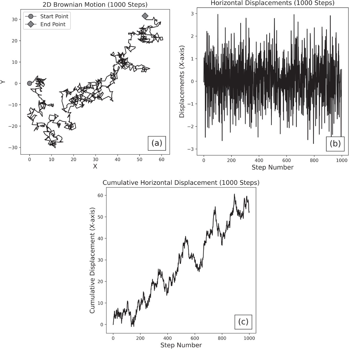
Figure 1.6 (a) The 2D position of a particle in a fluid, moving with Brownian motion. The particle begins at a coordinate of and drifts to a new location over 1,000 steps. (b) The horizontal displacements⁹ of the particle (i.e., the movements of the particle along the X‐axis over 1,000 steps). (c) The cumulative horizontal displacement of the particle over 1,000 steps.

Similarities are clear between price dynamics and Brownian motion, but this remains a highly simplified model of price dynamics. In reality, stock log returns are not normal and are typically skewed to the upside or downside, depending on the specific underlying. Additionally, the drift and volatility of a stock are not directly observable, and it cannot be experimentally confirmed whether or not these variables are constant. Stock volatility approximated with historical return data is rarely constant with time (a phenomenon known as heteroscedasticity). Stock returns are also not typically independent of one another across time (a phenomenon known as autocorrelation), which is a requirement for this model.

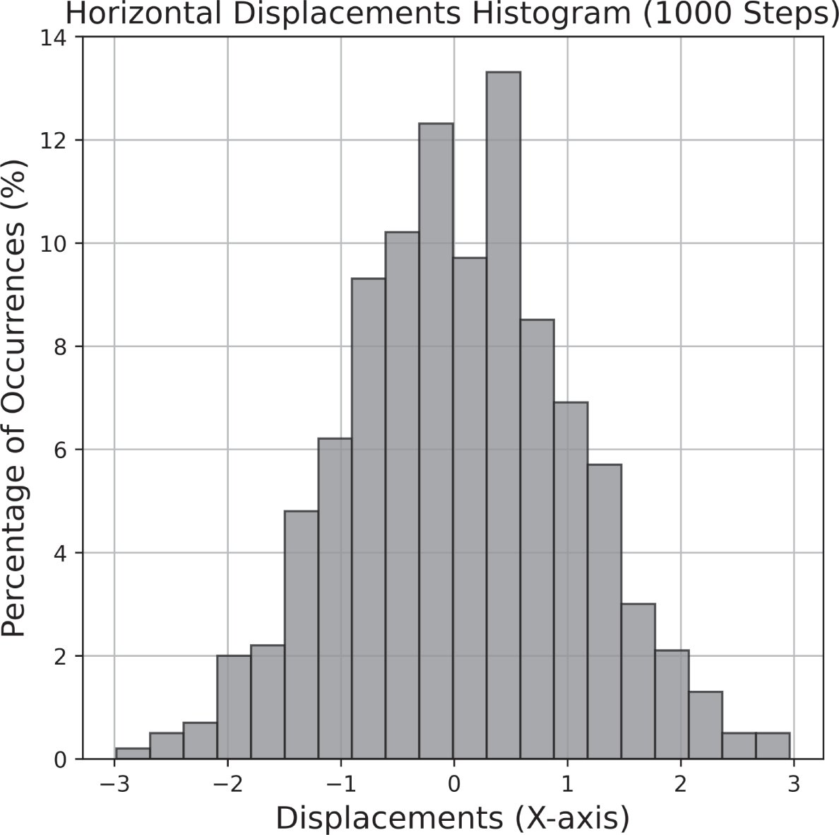
Figure 1.7 The distribution of the horizontal displacements of the particle over 1,000 steps. As characteristic of a Wiener process, the increments are normally distributed, have a mean of zero and variance (which equals 1 in this case). This figure indicates that horizontal step sizes between –1 and 1 are most common, and step sizes with a larger magnitude than 1 are less common.

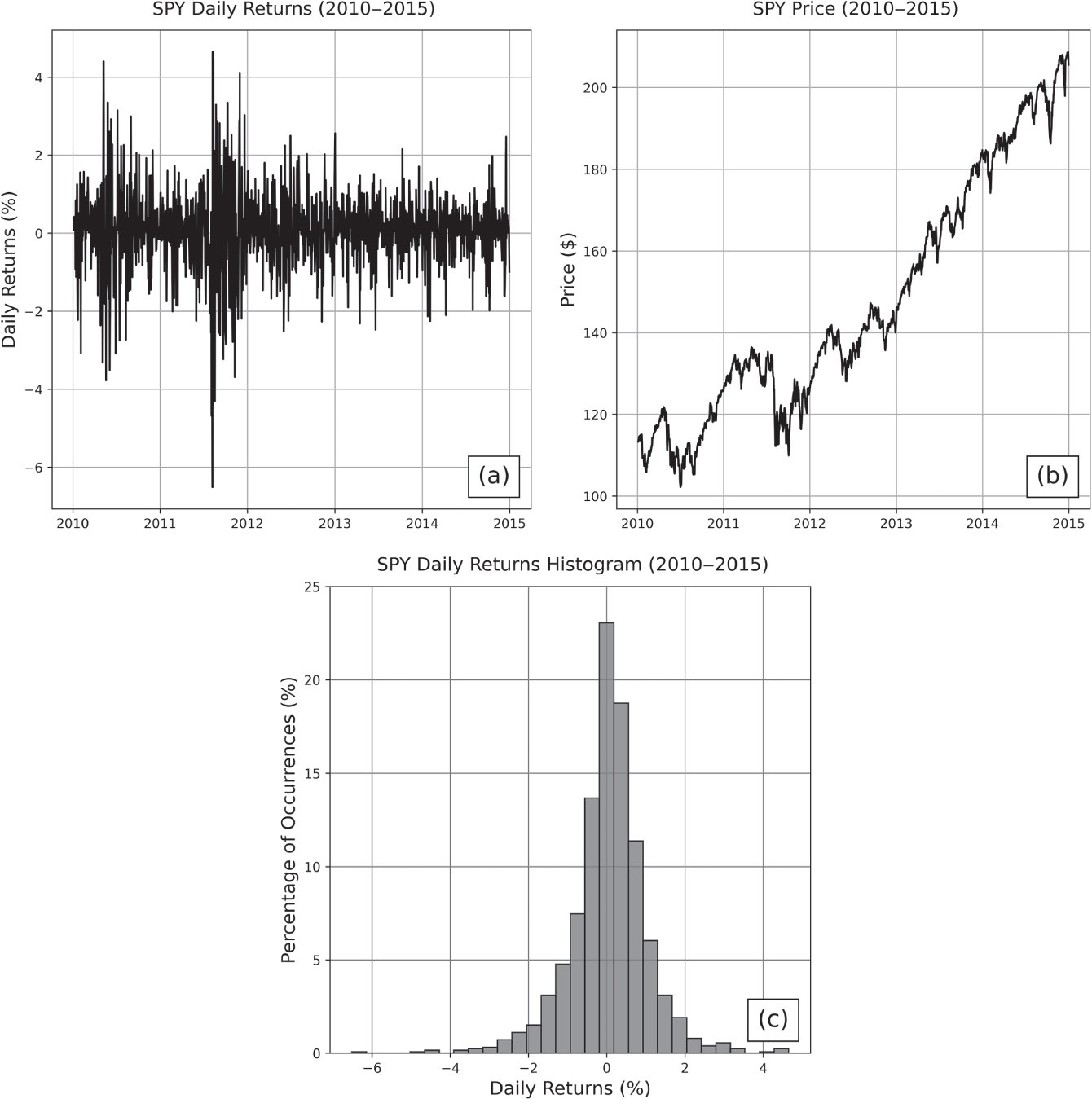
Figure 1.8 The (a) daily returns, (b) price, and (c) daily returns histogram for SPY from 2010–2015.

Although the normality assumption is not entirely accurate, making this simplification allows the development of the rest of this theoretical framework shown in the gray box. The formalism in the gray box is supplemental material for the mathematically inclined. The interpretation of the math, which is more significant, follows after. It should be noted that the Black‐Scholes model technically assumes that stock prices follow geometric Brownian motion, which is more accurate because price movements cannot be negative. Geometric Brownian motion is a slight modification of Brownian motion and requires that the logarithm of the signal follow Brownian motion rather than the signal itself. As it relates to price dynamics, this suggests that the log returns are normally distributed with constant drift (return rate) and volatility.¹⁰

For the price of a stock that follows a geometric Brownian motion, the dynamics of the asset price can be represented with the following stochastic differential equation:¹¹

(1.10)

where is the price of the stock at time t, is the Wiener process at time t , μ is a drift rate, and σ is the volatility of the stock. The drift rate and volatility of the stock are assumed to be constant, and it's important to reiterate that neither of these variables are directly observable. These constants can be approximated using the average return of a stock and the standard deviation of historical returns, but they can never be precisely known.

The equation states that each stock price increment is driven by a predictable amount of drift (with expected return ) and some amount of random noise . In other words, this equation has two components: one that models deterministic price trends and one that models probabilistic price fluctuations . The important takeaway from this observation is that inherent uncertainty is in the price of stock, represented with the contributions from the Wiener process. Because the increments of a Wiener process are independent of one another, it also is common to assume that the weak EMH holds at minimum, in addition to the normality of log returns.

Using this equation as a basis for the derivation, assuming a riskless options portfolio must earn the risk‐free rate, and rearranging terms, the Black‐Scholes equation follows:

(1.11)

where C is the price of a European call (with a dependence on S and t ), S is the price of the stock (with a dependence on t ), r is the risk‐free rate, and σ is the volatility of the stock. The Black‐Scholes formula can be calculated by solving the Black‐Scholes equation according to boundary conditions given by the payoff at expiration of European options. The formula, which provides the value of a European call option for a non‐dividend‐paying stock, is given by the following equation:

(1.12)

where is the value of the standard normal cumulative distribution function at and similarly for , T is the time that the option will expire ( is the duration of the contract), is the price of the stock at time t, K is the strike price of the option, and and are given by the following:

(1.13)

(1.14)

where σ is the volatility of the stock. If the equations seem gross, it's because they are.

Again, the purpose of this section is not to describe the underlying mechanics of the Black‐Scholes model in detail. Rather, Equations (1.10) through (1.14) are included to emphasize three important points.

1. There is inherent uncertainty in the price of stock. Stock price movements are also assumed to be independent of one another and log‐normally distributed.¹²

2. An estimate for the fair price of an option can be calculated according to the price of the stock, the volatility of the stock, the risk‐free rate, the duration of the contract, and the strike price.

3. The volatility of a stock, which plays an important role in estimating the risk of an asset and the valuation of an option, cannot be directly observed. This suggests that the “true risk” of an instrument can never be exactly known. Risk can only be approximated using a metric, such as historical volatility or the standard deviation of the historical returns over some timescale, typically matching the duration of the contract. Other than using a past‐looking metric, such as historical volatility to estimate the risk of an asset, one can also infer the risk of an asset from the price of its options.

As stated previously, the Black‐Scholes model only gives a theoretical estimate for the fair price of an option. Once the contract is traded on the options market, the price of the contract is often driven up or down depending on speculation and perceived risk. The deviation of an option's price from its theoretical value as a result of these external factors is indicative of implied volatility. When initially valuing an option, the historical volatility of the stock has been priced into the model. However, when the price of the option trades higher or lower than its theoretical value, this indicates that the perceived volatility of the underlying deviates from what is estimated by historical returns.

Implied volatility may be the most important metric in options trading. It is effectively a measure of the sentiment of risk for a given underlying according to the supply and demand for options contracts. For an example, suppose a non‐dividend‐paying stock currently trading at $100 per share has a historical 45‐day returns volatility of 20%. Suppose its call option with a 45‐day duration and a strike price of $105 is trading at $2 per share. Plugging these parameters into the Black‐Scholes model, this call option should theoretically be trading at $1 per share. However, demand for this position has increased the contract price significantly. For the model to return a call price of $2 per share, the volatility of this underlying would have to be 28% (assuming all else is constant). Therefore, although the historical volatility of the underlying is only 20%, the perceived risk of that underlying (i.e., the implied volatility) is actually 28%.

To conclude, the primary purpose of this section was not to dive into the math of the Black‐Scholes. These concepts were, instead, introduced to justify the following axioms that are foundational to this book:

● Profits cannot be made without risk.

● Stock log returns have inherent uncertainty and are assumed to follow a normal distribution.

● Stock price movements are independent across time (i.e., future price changes are independent of past price changes, requiring a minimum of the weak EMH).

● Options can theoretically be priced fairly based on the price of the stock, the volatility of the stock, the risk‐free rate, the duration of the contract, and the strike price.

● The volatility of an asset cannot be directly observed, only estimated using metrics like historical volatility or implied volatility.

The Greeks

Other than implied volatility, the Greeks are the most relevant metrics derived from the Black‐Scholes model. The Greeks are a set of risk measures, and each describes the sensitivity of an option's price with respect to changes in some variable. The most essential Greeks for options traders are delta , gamma , and theta .

Delta is one of the most important and widely used Greeks. It is a first‐order¹³ Greek that measures the expected change in the option price given a $1 increase in the price of the underlying (assuming all other variables stay constant). The equation is as follows:

(1.15)

where V is the price of the option (a call or a put) and S is the price of the underlying stock, noting that ∂ is the partial derivative. The value of delta ranges from –1 to 1, and the sign of delta depends on the type of position:

● Long stock: Δ is 1.

● Long call and short put: Δ is between 0 and 1.

● Long put and short call: Δ is between –1 and 0.

For example, the price of a long call option with a delta of 0.50 (denoted 50Δ because that is the total Δ for a one lot, or 100 shares of underlying) will increase by approximately $0.50 per share when the price of the underlying increases by $1. This makes intuitive sense because a long stock, a long call, and a short put are all bullish strategies, meaning they will profit when the underlying price increases. Similarly, because long puts and short calls are bearish, they will take a loss when the underlying price increases.

Delta has a sign and magnitude, so it is a measure of the degree of directional risk of a position. The sign of delta indicates the direction of the risk, and the magnitude of delta indicates the severity of exposure. The larger the magnitude of delta, the larger the profit and loss potential of the contract. This is because positions with larger deltas are closer to/deeper ITM and more sensitive to changes in the underlying price. A contract with a delta of 1.0 (100Δ ) has maximal directional exposure and is maximally ITM. 100Δ options behave like the stock price, as a $1 increase in the underlying creates a $1 increase in the option's price per share. A contract with a delta of 0.0 has no directional exposure and is maximally OTM. A 50Δ contract is defined as having the ATM strike.¹⁴

Because delta is a measure of directional exposure, it plays a large role when hedging directional risks. For instance, if a trader currently has a 50Δ position on and wants the position to be relatively insensitive to directional moves in the underlying, the trader could offset that exposure with the addition of 50 negative deltas (e.g., two 25Δ long puts). The composite position is called delta neutral.

Gamma is a second‐order Greek and a measure of the expected change in the option delta given a $1 change in the underlying price. Gamma is mathematically represented as follows:

(1.16)

As with delta, the sign of gamma depends on the type of position:

● Long call and long put: .

● Short call and short put: .

In other words, if there is a $1 increase in the underlying price, then the delta for all long positions will become more positive, and the delta for all short positions will become more negative. This makes intuitive sense because a $1 increase in the underlying pushes long calls further ITM, increasing the directional exposure of the contract, and it pushes long puts further OTM, decreasing the inverse directional exposure of the contract and bringing the negative delta closer to zero. The magnitude of gamma is highest for ATM positions and lower for ITM and OTM positions, meaning that delta is most sensitive to underlying price movements at –50Δ and 50Δ .

Awareness of gamma is critical when trading options, particularly when aiming for specific directional exposure. The delta of a contract is typically transient, so the gamma of a position gives a better indication of the long‐term directional exposure. Suppose traders wanted to construct a delta neutral position by pairing a short call (negative delta) with a short put (positive delta), and they are considering using 20Δ or 40Δ contracts (all other parameters identical). The 40Δ contracts are much closer to ATM (50Δ ) and have more profit potential than the 20Δ positions, but they also have significantly more gamma risk and are less likely to remain delta neutral in the long term. The optimal choice would then depend on how much risk traders are willing to accept and their profit goals. For traders with high profit goals and a large enough account to handle the large P/L swings and loss potential of the trade, the 40Δ contracts are more suitable.

Theta is a first‐order Greek that measures the expected P/L changes resulting from the decay of the option's extrinsic value (the difference between the current market price for the option and the intrinsic value of the option) per day. It is also commonly referred to as the time decay of the option. Theta is mathematically represented as follows:

(1.17)

where V is the price of the option (a call or a put) and t is time. The sign of theta depends on the type of position and is opposite gamma:

● Long call and long put: .

● Short call and short put: .

In other words, the time decay of the extrinsic value decreases the value of the long position and increases the value of the short position. For instance, a long call with a theta of –5 per one lot is expected to decline in value by $5 per day. This makes intuitive sense because the holders of the contract take gradual losses as their asset depreciates with time, a result of the value of the option converging to its intrinsic value as uncertainty dissipates. Because the extrinsic value of a contract decreases with time, the short side of the position profits with time and experiences positive time decay. The magnitude of theta is highest for ATM options and lower for ITM and OTM positions, all else constant.

There is a trade‐off between the gamma and theta of a position. For instance, a long call with the benefit of a large, positive gamma will also be subjected to a large amount of negative time decay. Consider these examples:

● Position 1: A 45 DTE, 16Δ call with a strike price of $50 is trading on a $45 underlying. The long position has a gamma of 5.4 and a theta of –1.3.

● Position 2: A 45 DTE, 44Δ call with a strike price of $50 is trading on a $49 underlying. The long position has a gamma of 7.9 and a theta of –2.2.

Compared to the first position, the second position has more gamma exposure, meaning that the contract delta (and the contract price) is more sensitive to changes in the underlying price and is more likely to move ITM. However, this position also comes with more theta decay, meaning that the extrinsic value also decreases more rapidly with time.

To conclude this discussion of the Black‐Scholes model and its risk measures, note that the outputs of all options pricing models should be taken with a grain of salt. Pricing models are founded on simplified assumptions of real financial markets. Those assumptions tend to become less representative in highly volatile market conditions when potential profits and losses become much larger. The assumptions and Greeks of the Black‐Scholes model can be used to form reasonable expectations around risk and return in most market conditions, but it's also important to supplement that framework with model‐free statistics.