Kitabı oxu: «SUGGESTIONS FOR ESTABLISHING A CHINA AND RUSSIA FREE TRADE ZONE»

Analysis of the trade effect of the China-Russia Free Trade Zone

1. Model introduction

The trade gravity model is used to analyze the trade flow between countries. It evolved from Newton's law of gravity in 1960. Tinbergen and Poyhonen were the first to apply the gravity model to the field of international trade. These two economists conducted a quantitative analysis on the trade between two countries. They believed that the scale of bilateral trade flows between the two countries is related to the respective economies of these two countries. The scale is directly proportional and inversely proportional to the spatial distance between the two countries. This analysis conclusion of Tinbergen and Poyhonen has opened up a new space for the study of international trade theory in the field of econometrics. Subsequently, as the research continued to deepen, more and more explanatory variables were brought into the model to meet the needs of research. For example,

economic factors, including per capita GDP, per capita national income, foreign direct investment, tariff rates, consumer price index, etc.;

geographic factors, including climate, territorial borders, etc.;

demographic factors, including language , Religion, population, etc.;

related political factors, including whether to sign a free trade agreement, whether to establish an FTA, whether it is a developed country, etc.

Because of its simple principles and strong data availability, the trade gravity model has gradually been widely used in the field of economics and has become one of the main empirical research tools for studying trade flows in international trade.

In 1962, the Dutch economist Jan Tinbergen summarized the basic form of the trade gravity model based on the universal gravitation formula, namely the trade gravity equation:

where Tij – represents the export of exporting country i to importing country j; A – a constant;

Yi – the GDP of country i;

Yj – the GDP of country j, is the product of the GDP of the two countries;

Dij – is the distance between country i and country j (is generally expressed by the distance between the capitals of the two countries).

The model is a non-linear model. Therefore, taking the natural logarithm on both sides of the formula becomes the linear form as follows:

2. Description of model data

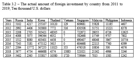
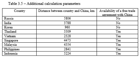
The data extracted in this article comes from the China Statistical Yearbook. The main trading member countries and regions selected are: Russia, India, South Korea, Thailand, Vietnam, Singapore, Malaysia, the Philippines and Indonesia. The time span selected in this article is from 2011 to 2019. The total bilateral trade and foreign direct investment data are from the China Statistical Yearbook. The data on GDP and GDP per capita are from the official website of the World Bank. The geographical distance is selected between the capitals of the two countries. The distance, the data comes from Google Earth, and the information on whether China has signed a free trade agreement with its trading partner countries comes from the official website of the China Free Trade Zone Service. See the table below for specific data:

3. Model construction and regression

Based on the status quo of bilateral trade between China and the world's major trading members and regions, this article analyzes the variables that affect the bilateral trade volume, and rationally introduces and removes relevant variables, so as to establish an economy that conforms to the bilateral trade between China and the world's major trading members and regions Correlation analysis between variables. Through the analysis of the correlation between these variables, it can be seen that there are certain correlations among variables such as economic aggregate, investment level, geographic distance, bordering, absolute value of per capita balance, and whether to sign a free trade agreement, and so on. It will make an intuitive and effective judgment on the economic, political, and geographic factors generated by the bilateral trade between China and the world's major trading member countries and the impact on the development of bilateral trade. Based on the analysis of the original trade gravity model and the selected indicators, the panel data model is constructed as follows:

where c – represents China;

p – represents the trading partner country;

y – represents the year.

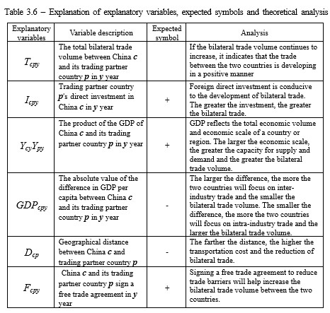
The explanation of specific explanatory variables is shown in Table 3.6.

Use the data collected in the China Statistical Yearbook to analyze the trade gravity model through the Stata software of econometrics:

It can be seen from Table 3.7 that, except for dummy variables, the standard deviation of each variable is extremely large, indicating that the sample data is extremely scattered, so in the following empirical steps, the above variables are processed logarithmically.

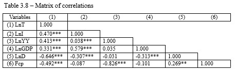
From Table 3.8 we can see the correlation between the two variables. The sign of the coefficient can reflect the positive or negative correlation of the two variables to a certain extent. *** means significant at the 99% confidence level, ** Indicates that it is significant at the 95% confidence level. It can be seen that the correlation between most indicators and the explained variable is very significant, indicating that the model is effective.

In the Hausman test, if the P value is greater than 0.1, the null hypothesis is accepted and the random effects model is selected. If the P value is less than 0.1, the null hypothesis is rejected and the fixed effects model is selected. The specific results are as follows:

– Chi-square test value is 3.02;

– P-value is 0.6969

According to the output result, the value of Hausman statistic is 3.02, and the corresponding P value is 0.6969, which means accepting the null hypothesis and establishing a random effects model.

Breusch and Pagan (1980) provided an LM test to test individual random effects. The original hypothesis is H0: = 0, and the alternative hypothesis is H1: ≠ 0. Through the LM test, we can know that the p value is 0.0000, which strongly rejects the null hypothesis, indicating that the original model should include the random disturbance item ui that reflects the individual characteristics, instead of using mixed regression, and choosing to use random effects regression.

Table shows the random effects regression results. From the data in the table, it can be seen that the R2 of the model is 0.686, and the model has a high degree of goodness of fit, indicating that the model setting is effective.

The following conclusions can be drawn from the results of the equation:

The p-value of the direct investment (LnI) of trading partner countries in China is 0.038, which is significant at the 95% confidence level, and the coefficient is 0.032, indicating that foreign direct investment is beneficial to the development of bilateral trade.

The explanatory variable has a product coefficient of 0.568 for the GDP of the two countries, indicating that the higher the GDP, the larger the economic scale and the larger the bilateral trade volume. Therefore, for every 1% increase in the logarithm of the product of the GDP of the two countries, the logarithm of the bilateral trade volume between the two countries will increase by 0.568%. It further shows that the increase in GDP of China and Russia, the increase in total economic volume and economic scale, and the increase in economic level have a significant promotion effect on the bilateral trade between the two countries.

The p-value of the distance between China and its trading partners (LnD) is 0.017, which is significant at the 95% confidence level, and the coefficient is - 0.709, indicating that the distance is negatively correlated with the bilateral trade volume. Although the Chinese capital Beijing is relatively far from the Russian capital Moscow, the Northeast region represented by Heilongjiang is very close to the Russian Far East. Strengthening trade cooperation between Northeast China and the Russian Far East will be more conducive to the expansion of China and Russia trade.

The p-value of the per capita GDP difference (LnGDP) between the trading partner country and China is 0.860, and there is no significant correlation under the random effects model.

The p-value of the dummy variable whether to sign a free trade agreement (F) is 0.076, which is significant at the 90% confidence level, and the coefficient is 0.604, indicating that the signing of a free trade agreement does promote the growth of bilateral trade volume, which also shows that China and Russia The establishment of a free trade zone will produce trade creation effects, further showing that the establishment of a China and Russia free trade zone has a positive role in promoting the economic development of China and Russia.